Measuring associations between non-numeric variables

It is often useful to know how strongly or weakly two variables are associated: do they vary together or are they essentially unrelated?  In the case of numerical variables, the best-known measure of association is the product-moment correlation coefficient introduced by Karl Pearson at the end of the nineteenth century.  For variables that are ordered but not necessarily numeric (e.g., Likert scale responses with levels like “strongly agree,” “agree,” “neither agree nor disagree,” “disagree” and “strongly disagree”), association can be measured in terms of the Spearman rank correlation coefficient.  Both of these measures are discussed in detail in Chapter 10 of Exploring Data in Engineering, the Sciences, and Medicine.  For unordered categorical variables (e.g., country, state, county, tumor type, literary genre, etc.), neither of these measures are applicable, but applicable alternatives do exist.  One of these is Goodman and Kruskal’s tau measure, discussed very briefly in Exploring Data (Chapter 10, page 492).  The point of this post is to give a more detailed discussion of this association measure, illustrating some of its advantages, disadvantages, and peculiarities.

A more complete discussion of Goodman and Kruskal’s tau measure is given in Agresti’s book Categorical Data Analysis, on pages 68 and 69.  It belongs to a family of categorical association measures of the general form:

            a(x,y) = [V(y) – E{V(y|x)}]/V(y)

where V(y) is a measure of the overall (i.e., marginal) variability of y and E{V(y|x)} is the expected value of the conditional variability V(y|x) of y given a fixed value of x, where the expectation is taken over all possible values of x.  These variability measures can be defined in different ways, leading to different association measures, including Goodman and Kruskal’s tau as a special case.  Agresti’s book gives detailed expressions for several of these variability measures, including the one on which Goodman and Kruskal’s tau is based, and an alternative expression for the overall association measure a(x,y) is given in Eq. (10.178) on page 492 of Exploring Data.  This association measure does not appear to be available in any current R package, but it is easily implemented as the following function:

GKtau <- function(x,y){

  #

  #  First, compute the IxJ contingency table between x and y

  #

  Nij = table(x,y,useNA="ifany")

  #

  #  Next, convert this table into a joint probability estimate

  #

  PIij = Nij/sum(Nij)

  #

  #  Compute the marginal probability estimates

  #

  PIiPlus = apply(PIij,MARGIN=1,sum)

  PIPlusj = apply(PIij,MARGIN=2,sum)

  #

  #  Compute the marginal variation of y

  #

  Vy = 1 - sum(PIPlusj^2)

  #

  #  Compute the expected conditional variation of y given x

  #

  InnerSum = apply(PIij^2,MARGIN=1,sum)

  VyBarx = 1 - sum(InnerSum/PIiPlus)

  #

  #  Compute and return Goodman and Kruskal's tau measure

  #

  tau = (Vy - VyBarx)/Vy

  tau

}

An important feature of this procedure is that it allows missing values in either of the variables x or y, treating “missing” as an additional level.  In practice, this is sometimes very important since missing values in one variable may be strongly associated with either missing values in another variable or specific non-missing levels of that variable.

An important characteristic of Goodman and Kruskal’s tau measure is its asymmetry: because the variables x and y enter this expression differently, the value of a(y,x) is not the same as the value of a(x,y), in general.  This stands in marked contrast to either the product-moment correlation coefficient or the Spearman rank correlation coefficient, which are both symmetric, giving the same association between x and y as that between y and x.  The fundamental reason for the asymmetry of the general class of measures defined above is that they quantify the extent to which the variable x is useful in predicting y, which may be very different than the extent to which the variable y is useful in predicting x.  Specifically, if x and y are statistically independent, then E{V(y|x)} = V(y) – i.e., knowing x does not help at all in predicting y – and this implies that a(x,y) = 0.  At the other extreme, if y is perfectly predictable from x, then E{V(y|x)} = 0, which implies that a(x,y) = 1.  As the examples presented next demonstrate, it is possible that y is extremely predictable from x, but x is only slightly predictable from y.

Specifically, consider the sequence of 400 random numbers, uniformly distributed between 0 and 1 generated by the following R code:

            set.seed(123)

            u = runif(400)

(Here, I have used the “set.seed” command to initialize the random number generator so repeated runs of this example will give exactly the same results.)  The second sequence is obtained by quantizing the first, rounding the values of u to a single digit:

            x = round(u,digits=1)

The plot below shows the effects of this coarse quantization: values of u vary continuously from 0 to 1, but values of x are restricted to 0.0, 0.1, 0.2, … , 1.0.  Although this example is simulation-based, it is important to note that this type of grouping of variables is often encountered in practice (e.g., the use of age groups instead of ages in demographic characterizations, blood pressure characterizations like “normal,” “borderline hypertensive,” etc. in clinical data analysis, or the recording of industrial process temperatures to the nearest 0.1 degree, in part due to measurement accuracy considerations and in part due to memory limitations of early data collection systems). 

In this particular case, because the variables x and u are both numeric, we could compute either the product-moment correlation coefficient or the Spearman rank correlation, obtaining the very large value of approximately 0.995 for either one, showing that these variables are strongly associated.  We can also apply Goodman and Kruskal’s tau measure here, and the result is much more informative.  Specifically, the value of a(u,x) is 1 in this case, correctly reflecting the fact that the grouped variable x is exactly computable from the original variable u.  In contrast, the value of a(x,u) is approximately 0.025, suggesting – again correctly – that the original variable u cannot be well predicted from the grouped variable x. 

To illustrate a case where the product-moment and rank correlation measures are not applicable at all, consider the following alphabetic re-coding of the variable x into an unordered categorical variable c:

            letters = c(“A”, “B”, “C”, “D”, “E”, “F”, “G”, “H”, “I”, “J”, “K”)

            c = letters[10*x+1]

In this case, both of the Goodman and Kruskal tau measures, a(x,c) and a(c,x), are equal to 1, reflecting the fact that these two variables are effectively identical, related via the non-numeric transformation given above. 

Being able to detect relationships like these can be extremely useful in exploratory data analysis where such relationships may be unexpected, particularly in the early stages of characterizing a dataset whose metadata – i.e., detailed descriptions of the variables included in the dataset – is absent, incomplete, ambiguous, or suspect.  As a real data illustration, consider the rent data frame from the R package gamlss.data, which has 1,969 rows, each corresponding to a rental property in Munich, and 9 columns, each giving a characteristic of that unit (e.g., the rent, floor space, year of construction, etc.).  Three of these variables are Sp, a binary variable indicating whether the location is considered above average (1) or not (0), Sm, another binary variable indicating whether the location is considered below average (1) or not (0), and loc, a three-level variable combining the information in these other two, taking the values 1 (below average), 2 (average), or 3 (above average).  The Goodman and Kruskal tau values between all possible pairs of these three variables are:

            a(Sm,Sp) = a(Sp,Sm) = 0.037

            a(Sm,loc) = 0.245 vs. a(loc,Sm) = 1

            a(Sp,loc) = 0.701 vs. a(loc,Sp) = 1

The first of these results – the symmetry of Goodman and Kruskal’s tau for the variables Sm and Sp – is a consequence of the fact that this measure is symmetric for any pair of binary variables.  In fact, the odds ratio that I have discussed in previous posts represents a much better way of characterizing the relationship between binary variables (here, the odds ratio between Sm and Sp is zero, reflecting the fact that a location cannot be both “above average” and “below average” at the same time).  The real utility of the tau measure here is that the second and third lines above show that the variables Sm and Sp are both re-groupings of the finer-grained variable loc. 

Finally, a more interesting exploratory application to this dataset is the following one.  Computing Goodman and Kruskal’s tau measure between the location variable loc and all of the other variables in the dataset – beyond the cases of Sm and Sp just considered – generally yields small values for the associations in either direction.  As a specific example, the association a(loc,Fl) is 0.001, suggesting that location is not a good predictor of the unit’s floor space in meters, and although the reverse association a(Fl,loc) is larger (0.057), it is not large enough to suggest that the unit’s floor space is a particularly good predictor of its location quality.  The same is true of most of the other variables in the dataset: they are neither well predicted by nor good predictors of location quality.  The one glaring exception is the rent variable R: although the association a(loc,R) is only 0.001, the reverse association a(R,loc) is 0.907, a very large value suggesting that location quality is quite well predicted by the rent.  The beanplot above shows what is happening here: because the variation in rents for all three location qualities is substantial, knowledge of the loc value is not sufficient to accurately predict the rent R, but these rent values do generally increase in going from below-average locations (loc = 1) to average locations (loc = 2) to above-average locations (loc = 3).  For comparison, the beanplots below show why the association with floor space is so much weaker: both the mean floor space in each location quality group and the overall range of these values are quite comparable, implying that neither location quality can be well predicted from floor space nor vice versa.

The asymmetry of Goodman and Kruskal’s tau measure is disconcerting at first because it has no counterpart in better-known measures like the product-moment correlation coefficient between numerical variables, Spearman’s rank correlation coefficient between ordinal variables, or the odds ratio between binary variables.  One of the points of this post has been to demonstrate how this unusual asymmetry can be useful in practice, distinguishing between the ability of one variable x to predict another variable y, and the reverse case.

Computing Odds Ratios in R

In my last post, I discussed the use of odds ratios to characterize the association between edibility and binary mushroom characteristics for the mushrooms characterized in the UCI mushroom dataset.  I did not, however, describe those computations in detail, and the purpose of this post is to give a brief discussion of how they were done.  That said, I should emphasize that the primary focus of this blog is not R programming per se, but rather the almost limitless number of things that R allows you to do in the realm of exploratory data analysis.  For more detailed discussions of the mechanics of R programming, two excellent resources are The R Book by Michael J. Crawley, and Modern Applied Statistics with S (Statistics and Computing) by W.N. Venables and B.D. Ripley.

As a reminder, I discuss the odds ratio in Chapter 13 of Exploring Data in Engineering, the Sciences, and Medicine, which may be viewed as an association measure between binary variables.  As I discussed last time, for two binary variables, x and y, each taking the values 0 and 1, the odds ratio is defined on the basis of the following four numbers:

            N₀₀ = the number of data records with x = 0 and y = 0

            N₀₁ = the number of data records with x = 0 and y = 1

            N₁₀ = the number of data records with x = 1 and y = 0

            N₁₁ = the number of data records with x = 1 and y = 1

Specifically, the odds ratio is given by the following expression:

OR = N₀₀ N₁₁ / N₀₁ N₁₀

Similarly, confidence intervals for the odds ratio are easily constructed by appealing to the asymptotic normality of log OR, which has a limiting variance given by the square root of the sum of the reciprocals of these four numbers.  The R procedure oddsratioWald.proc available from the companion website for Exploring Data computes the odds ratio and the upper and lower confidence limits at a specified level alpha from these four values:

oddsratioWald.proc <- function(n00, n01, n10, n11, alpha = 0.05){

  #

  #  Compute the odds ratio between two binary variables, x and y,

  #  as defined by the four numbers nij:

  #

  #    n00 = number of cases where x = 0 and y = 0

  #    n01 = number of cases where x = 0 and y = 1

  #    n10 = number of cases where x = 1 and y = 0

  #    n11 = number of cases where x = 1 and y = 1

  #

  OR <- (n00 * n11)/(n01 * n10)

  #

  #  Compute the Wald confidence intervals:

  #

  siglog <- sqrt((1/n00) + (1/n01) + (1/n10) + (1/n11))

  zalph <- qnorm(1 - alpha/2)

  logOR <- log(OR)

  loglo <- logOR - zalph * siglog

  loghi <- logOR + zalph * siglog

  #

  ORlo <- exp(loglo)

  ORhi <- exp(loghi)

  #

  oframe <- data.frame(LowerCI = ORlo, OR = OR, UpperCI = ORhi, alpha = alpha)

  oframe

}

Including “alpha = 0.05” in the parameter list fixes the default value for alpha at 0.05, which yields the 95% confidence intervals for the computed odds ratio, based on the Wald approximation described above.  An important practical point is that these intervals become infinitely wide if any of the four numbers N_ij are equal to zero; also, note that in this case, the computed odds ratio is either zero or infinite.  Finally, it is worth noting that if the numbers N_ij are large enough, the procedure just described can encounter numerical overflow problems (i.e., the products in either the numerator or the denominator become too large to be represented in machine arithmetic).  If this is a possibility, a better alternative is to regroup the computations as follows:

OR = (N₀₀ / N₀₁) x (N₁₁ / N₁₀ )

To use the routine just described, it is necessary to have the four numbers defined above, which form the basis for a two-by-two contingency table.  Because contingency tables are widely used in characterizing categorical data, these numbers are easily computed in R using the table command.  As a simple example, the following code reads the UCI mushroom dataset and generates the two-by-two contingency table for the EorP and GillSize attributes:

> mushrooms <- read.csv("mushroom.csv")

>

> table(mushrooms$EorP, mushrooms$GillSize)

  

       b    n

  e 3920  288

  p 1692 2224

>

>

(Note that the first line reads the csv file containing the mushroom data; for this command to work as shown, it is necessary for this file to be in the working directory.  Alternatively, you can change the working directory using the setwd command.) 

To facilitate the computation of odds ratios, the following preliminary procedure combines the table command with the oddsratioWald.proc procedure, allowing you to compute the odds ratio and its level-alpha confidence interval from the two-level variables directly:

TableOR.proc00 <- function(x,y,alpha=0.05){

  #

  xtab <- table(x,y)

  n00 <- xtab[1,1]

  n01 <- xtab[1,2]

  n10 <- xtab[2,1]

  n11 <- xtab[2,2]

  oddsratioWald.proc(n00,n01,n10,n11,alpha)

}

The primary disadvantage of this procedure is that it doesn’t tell you which levels of the two variables are being characterized by the computed odds ratio.  In fact, this characterization describes the first level of each of these variables, and the following slight modification makes this fact explicit:

TableOR.proc <- function(x,y,alpha=0.05){

   #

   xtab <- table(x,y)

   n00 <- xtab[1,1]

   n01 <- xtab[1,2]

   n10 <- xtab[2,1]

   n11 <- xtab[2,2]

   #

   outList <- vector("list",2)

   outList[[1]] <- paste("Odds ratio between the level [",dimnames(xtab)[[1]][1],"] of the first variable and the level [",dimnames(xtab)[[2]][1],"] of the second variable:",sep=" ")

   outList[[2]] <- oddsratioWald.proc(n00,n01,n10,n11,alpha)

   outList

 }

Specifically, I have used the fact that the dimension names of the 2x2 table xtab correspond to the levels of the variables x and y, and I have used the paste command to include these values in a text string displayed to the user.  (I have enclosed the levels in square brackets to make them stand out from the surrounding text, particularly useful here since the levels are coded as single letters.)  Applying this procedure to the mushroom characteristics EorP and GillSize yields the following results:

> TableOR.proc(mushrooms$EorP, mushrooms$GillSize)

[[1]]

[1] "Odds ratio between the level [ e ] of the first variable and the level [ b ] of the second variable:"

[[2]]

   LowerCI       OR  UpperCI alpha

1 15.62615 17.89073 20.48349  0.05

>

Almost certainly, the formatting I have used here could be improved – probably a lot – but the key point is to provide a result that is reasonably complete and easy to interpret. 

Finally, I noted in my last post that if we are interested in using odds ratios to compare or rank associations, it is useful to code the levels so that the computed odds ratio is larger than 1.  In particular, note that applying the above procedure to characterize the relationship between edibility and the Bruises characteristic yields:

> TableOR.proc(mushrooms$EorP, mushrooms$Bruises)

[[1]]

[1] "Odds ratio between the level [ e ] of the first variable and the level [ f ] of the second variable:"

[[2]]

     LowerCI        OR   UpperCI alpha

1 0.09014769 0.1002854 0.1115632  0.05

>

It is clear from these results that both Bruises and GillSize exhibit odds ratios with respect to mushroom edibility that are significantly different from the neutral value 1 (i.e., the 95% confidence interval excludes the value 1 in both cases), but it is not obvious which variable has the stronger association, based on the available data.  The following procedure automatically restructures the computation so that the computed odds ratio is larger than or equal to 1, allowing us to make this comparison:

AutomaticOR.proc <- function(x,y,alpha=0.05){

  #

   xtab <- table(x,y)

   n00 <- xtab[1,1]

   n01 <- xtab[1,2]

   n10 <- xtab[2,1]

   n11 <- xtab[2,2]

   #

   rawOR <- (n00*n11)/(n01*n10)

   if (rawOR < 1){

     n01 <- xtab[1,1]

     n00 <- xtab[1,2]

     n11 <- xtab[2,1]

     n10 <- xtab[2,2]

     iLevel <- 2

   }

   else{

     iLevel <- 1

   }

   outList <- vector("list",2)

   outList[[1]] <- paste("Odds ratio between the level [",dimnames(xtab)[[1]][1],"] of the first variable and the level [",dimnames(xtab)[[2]][iLevel],"] of the second variable:",sep=" ")

   outList[[2]] <- oddsratioWald.proc(n00,n01,n10,n11,alpha)

   outList

 }

Note that this procedure first constructs the 2x2 table on which everything is based and then computes the odds ratio in the default coding: if this value is smaller than 1, the coding of the second variable (y) is reversed.  The odds ratio and its confidence interval are then computed and the levels of the variables used in computing it are presented as before.  Applying this procedure to the Bruises characteristic yields the following result, from which we can see that GillSize appears to have the stronger association, as noted last time:

> AutomaticOR.proc(mushrooms$EorP, mushrooms$Bruises)

[[1]]

[1] "Odds ratio between the level [ e ] of the first variable and the level [ t ] of the second variable:"

[[2]]

   LowerCI       OR  UpperCI alpha

1 8.963532 9.971541 11.09291  0.05

>

Well, that’s it for now.  Next time, I will come back to the question of how we should expect interestingness measures to be distributed and whether those expectations are met in practice.

Measuring association using odds ratios

In my last two posts, I have used the UCI mushroom dataset to illustrate two things.  The first was the use of interestingness measures to characterize categorical variables, and the second was the use of binary confidence intervals to visualize the relationship between a categorical predictor variable and a binary response variable.  This second approach can be applied to categorical predictors having any number of levels, but in the case of a binary (i.e., two-level) predictor, an attractive alternative is to measure their association with odds ratios.  The objective of this post is to illustrate this idea and highlight a few important details.

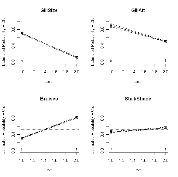
The above plots show the binomial confidence intervals discussed last time for four different binary mushroom characteristics: GillSize (upper left), GillAtt (upper right), Bruises (lower left), and StalkShape (lower right).  Specifically, these plots show the estimated probability that mushrooms with each of the two possible values for these variables are edible.  Thus, the upper left plot shows that mushrooms with GillSize characteristic “b” (“broad”) are much more likely to be edible than mushrooms with GillSize characteristic “n” (“narrow”).  The other three plots have analogous interpretations: mushrooms with GillAtt value “a” (“attached”) are more likely to be edible than those with value “f” (“free”), mushrooms with bruises (Bruises value “t”) are more likely to be edible than those without (Bruises value “f”), and mushrooms with StalkShape value “t” (“tapering”) are slightly more likely to be edible than those with value “e” (“enlarging”).   Also, while the smaller slopes for GillAtt and StalkShape suggest this association is weaker for these variables than for GillSize, where the slope appears much larger, it would be nice to have a quantitative measure of this degree of association that we could compare directly.  This is particularly the case for GillSize and Bruises, where both associations appear to be reasonably strong, but since the reference lines run in opposite directions on the plots, it is difficult to reliably compare the slopes on the basis of appearance alone.

The odds ratio provides a simple quantitative association measure for these variables that allows us to make these comparisons directly.  I discuss the odds ratio in Chapter 13 of  Exploring Data in Engineering, the Sciences, and Medicine in connection with the practical implications of data type (e.g., numerical versus categorical data).  The odds ratio may be viewed as an association measure between binary variables, and it is defined as follows.  For simplicity, suppose x and y are two binary variables of interest and assume that they are coded so that they each take the values 0 or 1 – this assumption is easily relaxed, as discussed below, but it simplifies the basic description of the odds ratio.  Next, define the following four numbers:

            N₀₀ = the number of data records with x = 0 and y = 0

            N₀₁ = the number of data records with x = 0 and y = 1

            N₁₀ = the number of data records with x = 1 and y = 0

            N₁₁ = the number of data records with x = 1 and y = 1

The odds ratio is defined in terms of these four numbers as

OR = N₀₀ N₁₁ / N₀₁ N₁₀

Since all of the four numbers appearing in this ratio are nonnegative, it follows that the odds ratio is also nonnegative and can assume any value between 0 and positive infinity.  Further, if x and y are two statistically independent binary random variables, it can be shown that the odds ratio is equal to 1.  Values greater than 1 imply that records with y = 1 are more likely to have x = 1 than x = 0, and similarly, that records with y = 0 are more likely to have x = 0 than x = 1; in other words, OR > 1 implies that the variables x and y are more likely to agree than they are to disagree.  Conversely, odds ratio values less than 1 imply that the variables x and y are more likely to disagree: records with y = 1 are more likely to have x = 0 than x = 1, and those with y = 0 are more likely to have x = 1 than x = 0.

Often – as in the mushroom dataset – the binary variables are not coded as 0 or 1, but instead as two different categorical values.  As a specific example, the binary response variable considered last time – the edibility variable EorP – assumes the values “e” (for “edible”) or “p” (for “poisonous” or “non-edible”).  In the results presented here, we recode EorP to have the values 1 for edible mushrooms and 0 for non-edible mushrooms.  For the mushroom characteristic GillSize shown in the upper left plot above, suppose we initially code the value “b” (“broad”) as 0 and the value “n” (“narrow”) as 1.  This choice is arbitrary – we could equally well code “b” as 1 and “n” as zero – and its practical consequences are explored further below.  For the coding just described, the odds ratio between mushroom edibility (EorP) and gill size (GillSize) is 0.056.  Since this number is substantially smaller than 1, it suggests that edible mushrooms (y = 1) are unlikely to be associated with narrow gills (x = 1), a result that is consistent with the appearance of the upper left plot above. 

An important practical issue in interpreting odds ratios is that of how much smaller or larger than 1 the computed odds ratio should be to be regarded as evidence for a “significant” association between the variables x and y.  That is, since we are computing this ratio from uncertain data, we need a measure of precision for the odds ratio, like the binomial confidence intervals discussed in my last post: e.g., how much does the odds ratio change if some mushrooms previously declared edible is reclassified as poisonous, or if some additional mushrooms are added to our dataset?  Fortunately, confidence intervals for the odds ratio are easily constructed.  In his book Categorical Data Analysis (Wiley Series in Probability and Statistics), Alan Agresti notes that confidence intervals for the odds ratio can be computed directly by appealing to the fact that the odds ratio estimator is asymptotically normal, approaching a Gaussian distribution in the limit of large sample sizes.  He does not give explicit results for these direct confidence intervals, however, because he does not recommend them.  Instead, Agresti advocates the construction of confidence intervals for the log of the odds ratio and transforming them back to get upper and lower confidence limits for the odds ratio itself.  This recommendation rests primarily on three practical points: first, that the log of the odds ratio approaches normality faster than the odds ratio itself does, so this approach yields more accurate confidence intervals; second, this approach guarantees a positive lower confidence limit for the odds ratio, which is not the case for the direct approach; and, third, the same result can be used to compute confidence intervals for both the odds ratio and its reciprocal, a result that is again not true for the direct approach and that will be useful in the discussion presented below. 

For the gill size example, Agresti’s recommended procedure yields a 95% confidence interval between 0.049 and 0.064.  Since this interval does not include the value 1, we conclude that there is evidence to support an association between a mushroom’s gill size and its edibility, at least for mushrooms in the UCI dataset. Applying this procedure to the GillAtt characteristic shown in the upper right plot above yields an estimated odds ratio of 0.097 with a 95% confidence interval between 0.059 and 0.157.  Again, the fact that this interval does not include 1 supports the idea that the GillAtt characteristic is associated with edibility (again, for the mushrooms considered here), but the fact that this odds ratio is larger (i.e., closer to the neutral value 1) also suggests that this association is weaker than that between edibility and the GillShape characteristic.  Again, this result is in agreement with the visual appearance of the upper right plot above, relative to that of the upper left plot.  The advantage of the odds ratio over these plots is that it provides a quantitative measure that can be used to make more objective comparisons, removing the subjective visual judgment required in comparing plots.

Applying this procedure to the Bruises variable yields an odds ratio of 9.972, with a 95% confidence interval from 8.963 to 11.093.  The fact that these values are larger than 1 implies that mushrooms whose bruise characteristics have been coded as 1 (here, “t” for “true” or “bruised”) are more likely to be edible than those whose characteristics have been coded as 0 (here, “f” for “false” or “not bruised”).  As noted above, this coding is arbitrary, as were the earlier assignments.  An extremely useful observation is that if we reverse this assignment – i.e., for this example, if we code “bruised” as 0 and “not bruised” as 1 – we simply exchange the numbers N₀₀ with N₁₀ and also the numbers N₁₁ with N₀₁.  The effect of these exchanges on the odds ratio is a reciprocal transformation:

            OR = N₀₀N₁₁/N₀₁N₁₀ -> N₁₀N₀₁/N₁₁N₀₀ = 1/OR

This observation provides a simple basis for comparing results like those for GillSize where the odds ratio is less than 1 with those for Bruises where the odds ratio is greater than 1.  As with the visual comparisons discussed above, it is not obvious from the odds ratios computed so far which of these variables is more strongly associated with mushroom edibility.  Reversing the coding for GillSize so that “b” is coded as 1 and “n” is coded as 0 changes the odds ratio from 0.059 to 1/0.059 = 17.857.  Since this number is larger than the odds ratio of 9.972 for Bruises, we can conclude that GillSize is more strongly associated with edibility – i.e., it is a better predictor of edibility for the mushrooms considered here – than Bruises, at least for this dataset. 

In fact, the same trick can be applied to the confidence intervals, illustrating the third advantage noted above for Agresti’s preferred approach to constructing these intervals.  Specifically, the asymptotically normal approximation says that the log of the odds ratio has a mean of log OR and a standard deviation S that can be simply computed from the four numbers N₀₀, N₀₁, N₁₀, and N₁₁.  Since the Gaussian distribution is symmetric about its mean and log(1/OR) = - log(OR), it follows that the log of the reciprocal odds ratio has the same approximate standard deviation S as log(OR).  In practical terms, this means that if we reverse the coding of our binary predictor variables, it is a simple matter to compute new confidence intervals as follows:

            New lower CI = 1/Old upper CI

            New odds ratio = 1/Old odds ratio

            New upper CI = 1/Old lower CI

(Note here that because the reciprocal transformation is order-reversing, the transformation of the lower confidence limit yields the new upper confidence limit, and vice-versa; for a more detailed discussion of order-preserving and order-reversing transformations in general and the reciprocal transformation in particular, refer to Chapter 12 of Exploring Data.)

Applying these transformation results to the odds ratio for Bruises yields a new odds ratio of 0.100, with a 95% confidence interval from 0.090 to 0.112, which we can now compare with the earlier results for GillSize and GillAtt.  Alternatively, if we reverse the coding of the results for GillSize and GillAtt, we obtain odds ratios that are larger than 1 between edibility and “the more edible value” of each of these mushroom characteristics.  This has the advantage of giving us a sequences of odds ratios, all larger than 1, with the largest value suggestive of the strongest association between each mushroom characteristic variable and edibility.  For the four mushroom characteristics shown in the above four plots, this approach yields the following odds ratios and their 95% confidence intervals:

            GillSize:       Lower CI = 15.625,  OR = 17.857,  Upper CI = 20.408

            GillAtt:        Lower CI =   6.369,  OR = 10.309,  Upper CI = 16.949

            Bruises:       Lower CI =   8.963,  OR =  9.972,   Upper CI = 11.093

            StalkShape: Lower CI =   1.384,  OR = 1.512,    Upper Ci = 1.651

These results suggest that, of these four variables, the best predictor of mushroom edibility is GillSize, followed by GillAtt as second-best, then Bruises, and finally StalkShape as least predictive.  These conclusions are probably the same as we would draw based on a careful comparison of the plots shown above, but the odds ratios computed in the way just described lead us to these conclusions much more directly.

Finally, it is important to make three points.  First, as I have noted before – but the point is important enough to bear repeating – the associations described here between these binary mushroom characteristics and edibility are based entirely on the UCI mushroom dataset.  Thus, these conclusions are only as representative of mushrooms in general or in any particular setting as the UCI mushroom dataset is representative of this larger and/or different mushroom population.  In particular, mushrooms from other locales or unusual environments may exhibit different relationships between edibility and gill size or other characteristics than the UCI mushrooms do.  The second key point is that the results presented here only attempt to assess the predictability of a single binary mushroom characteristic in isolation.  To get a more complete picture of the relationship between mushroom characteristics and edibility, it is necessary to explore more general multivariate analysis techniques like logistic regression.  More about that later.  Last but not least, the third point is that I realized in reviewing this post before I issued it that I hadn't included any actual R code to compute odds ratios.  In my next post, I will remedy this problem, giving a detailed view of how the numbers presented here were obained.