In my last post, I discussed the Hampel filter, a useful moving window nonlinear data cleaning filter that is available in the R package pracma. In this post, I briefly discuss this moving window filter in a little more detail, focusing on two important practical points: the choice of the filter’s local outlier detection threshold, and the question of how to initialize moving window filters. This second point is particularly important here because the pracma package initializes the Hampel filter in a particularly appropriate way, but doesn’t do such a good job of initializing the Savitzky-Golay filter, a linear smoothing filter that is popular in physics and chemistry. Fortunately, this second difficulty is easy to fix, as I demonstrate here.
Recall from my last post that the Hampel filter is a moving window implementation of the Hampel identifier, discussed in Chapter 7 of Exploring Data in Engineering, the Sciences, and Medicine. In particular, this procedure – implemented as outlierMAD in the pracma package – is a nonlinear data cleaning filter that looks for local outliers in a time-series or other streaming data sequence, replacing them with a more reasonable alternative value when it finds them. Specifically, this filter may be viewed as a more effective alternative to a “local three-sigma edit rule” that would replace any data point lying more than three standard deviations from the mean of its neighbors with that mean value. The difficulty with this simple strategy is that both the mean and especially the standard deviation are badly distorted by the presence of outliers in the data, causing this data cleaning procedure to often fail completely in practice. The Hampel filter instead uses the median of neighboring observations as a reference value, and the MAD scale estimator as an alternative measure of distance: that is, a data point is declared an outlier and replaced if it lies more than some number t of MAD scale estimates from the median of its neighbors; the replacement value used in this procedure is the median.
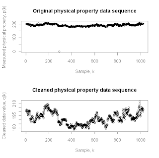
More specifically, for each observation in the original data sequence, the Hampel filter constructs a moving window that includes the K prior points, the data point of primary interest, and the K subsequent data points. The reference value used for the central data point is the median of these 2K+1 successive observations, and the MAD scale estimate is computed from these same observations to serve as a measure of the “natural local spread” of the data sequence. If the central data point lies more than t MAD scale estimate values from the median, it is replaced with the median; otherwise, it is left unchanged. To illustrate the performance of this filter, the top plot above shows the sequence of 1024 successive physical property measurements from an industrial manufacturing process that I also discussed in my last post. The bottom plot in this pair shows the results of applying the Hampel filter with a window half-width parameter K=5 and a threshold value of t = 3 to this data sequence. Comparing these two plots, it is clear that the Hampel filter has removed the glaring outlier – the value zero – at observation k = 291, yielding a cleaned data sequence that varies over a much narrower (and, at least in this case, much more reasonable) range of possible values. What is less obvious is that this filter has also replaced 18 other data points with their local median reference values.
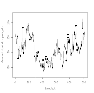
The above plot shows the original data sequence, but on approximately the same range as the cleaned data sequence so that the glaring outlier at k = 291 no longer dominates the figure. The large solid circles represent the 18 additional points that the Hampel filter has declared to be outliers and replaced with their local median values. This plot was generated using the Hampel filter implemented in the outlierMAD command in the pracma package, which has the following syntax:
outlierMAD(x,k)
where x is the data sequence to be cleaned and k is the half-width that defines the moving data window on which the filter is based. Here, specifying k = 5 results in an 11-point moving data window. Unfortunately, the threshold parameter t is hard-coded as 3 in this pracma procedure, which has the following code:
outlierMAD <- function (x, k){
n <- length(x)
y <- x
L <- 1.4826
t0 <- 3
for (i in (k + 1):(n - k)) {
x0 <- median(x[(i - k):(i + k)])
S0 <- L * median(abs(x[(i - k):(i + k)] - x0))
if (abs(x[i] - x0) > t0 * S0) {
y[i] <- x0
}
}
list(y = y, ind = ind
}
Note that it is a simple matter to create your own version of this filter, specifying the threshold (here, the variable t0) to have a default value of 3, but allowing the user to modify it in the function call. Specifically, the code would be:
HampelFilter <- function (x, k,t0=3){
n <- length(x)
y <- x
L <- 1.4826
for (i in (k + 1):(n - k)) {
x0 <- median(x[(i - k):(i + k)])
S0 <- L * median(abs(x[(i - k):(i + k)] - x0))
if (abs(x[i] - x0) > t0 * S0) {
y[i] <- x0
}
}
list(y = y, ind = ind
}
The advantage of this modification is that it allows you to explore the influence of varying the threshold parameter. Note that increasing t0 makes the filter more forgiving, allowing more extreme local fluctuations to pass through the filter unmodified, while decreasing t0 makes the filter more aggressive, declaring more points to be local outliers and replacing them with the appropriate local median. In fact, this filter remains well-defined even for t0 = 0, where it reduces to the median filter, popular in nonlinear digital signal processing. John Tukey – the developer or co-developer of many useful things, including the fast Fourier transform (FFT) – introduced the median filter at a technical conference in 1974, and it has profoundly influenced subsequent developments in nonlinear digital filtering. It may be viewed as the most aggressive limit of the Hampel filter and, although it is quite effective in removing local outliers, it is often too aggressive in practice, introducing significant distortions into the original data sequence. This point may be seen in the plot below, which shows the results of applying the median filter (i.e., the HampelFilter procedure defined above with t0=0) to the physical property dataset. In particular, the heavy solid line in this plot shows the behavior of the first 250 points of the median filtered sequence, while the lighter dotted line shows the corresponding results for the Hampel filter with t0=3. Note the “clipped” or “blocky” appearance of the median filtered results, compared with the more irregular local variation seen in the Hampel filtered results. In many applications (e.g., fitting time-series models), the less aggressive Hampel filter gives much better overall results.
The other main issue I wanted to discuss in this post is that of initializing moving window filters. The basic structure of these filters – whether they are nonlinear types like the Hampel and median filters discussed above, or linear types like the Savitzky-Golay filter discussed briefly below – is built on a moving data window that includes a central point of interest, prior observations and subsequent observations. For a symmetric window that includes K prior and K subsequent observations, this window is not well defined for the first K or the last K observations in the data sequence. These points must be given special treatment, and a very common approach in the digital signal processing community is to extend the original sequence by appending K additional copies of the first element to the beginning of the sequence and K additional copies of the last element to the end of the sequence. The pracma implementation of the Hampel filter procedure (outlierMAD) takes an alternative approach, one that is particularly appropriate for data cleaning filters. Specifically, procedure outlierMAD simply passes the first and last K observations unmodified from the original data sequence to the filter output. This would also seem to be a reasonable option for smoothing filters like the linear Savitzky-Golay filter discussed next.
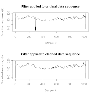
As noted, this linear smoothing filter is popular in chemistry and physics, and it is implemented in the pracma package as procedure savgol. For a more detailed discussion of this filter, refer to the treatment in the book Numerical Recipes, which the authors of the pracma package cite for further details (Section 14.8). Here, the key point is that this filter is a linear smoother, implemented as the convolution of the input sequence with an impulse response function (i.e., a smoothing kernel) that is constructed by the savgol procedure. The above two plots show the effects of applying this filter with a total window width of 11 points (i.e., the same half-width K = 5 used with the Hampel and median filters), first to the raw physical property data sequence (upper plot), and then to the sequence after it has been cleaned by the Hampel filter (lower plot). The large downward spike at k = 291 in the upper plot reflects the impact of the glaring outlier in the original data sequence, illustrating the practical importance of removing these artifacts from a data sequence before applying smoothing procedures like the Savitzky-Golay filter. Both the upper and lower plots exhibit similarly large spikes at the beginning and end of the data sequence, however, and these artifacts are due to the moving window problem noted above for the first K and the last K elements of the original data sequence. In particular, the filter implementation in the savgol procedure does not apply the sequence extension procedure discussed above, and this fact is responsible for these artifacts appearing at the beginning and end of the smoothed data sequence.
It is extremely easy to correct this problem, adopting the same philosophy the package uses for the outlierMAD procedure: simply retain the first and last K elements of the original sequence unmodified. The procedure SGwrapper listed below does this after the fact, calling the savgol procedure and then replacing the first and last K elements of the filtered sequence with the original sequence values:
SGwrapper <- function(x,K,forder=4,dorder=0){
#
n = length(x)
fl = 2*K+1
y = savgol(x,fl,forder,dorder)
if (dorder == 0){
y[1:K] = x[1:K]
y[(n-K):n] = x[(n-K):n]
}
else{
y[1:K] = 0
y[(n-K):n] = 0
}
y
}
Before showing the results obtained with this procedure, it is important to note two points. First, the moving window width parameter fl required for the savgol procedure corresponds to fl = 2K+1 for a half-width parameter K. The procedure SGwrapper instead requires K as its passing parameter, constructing fl from this value of K. Second, note that in addition to serving as a smoother, the Savitzky-Golay filter family can also be used to estimate derivatives (this is tricky since differentiation filters are incredible noise amplifiers, but I’ll talk more about that in another post). In the savgol procedure, this is accomplished by specifying the parameter dorder, which has a default value of zero (implying smoothing), but which can be set to 1 to estimate the first derivative of a sequence, 2 for the second derivative, etc. In these cases, replacing the first and last K elements of the filtered sequence with the original data sequence elements is not reasonable: in the absence of any other knowledge, a better default derivative estimate is zero, and the SGwrapper procedure listed above does this.
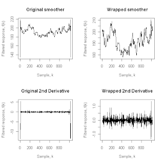
The four plots shown above illustrate the differences between the original savgol procedure (the left-hand plots) and those obtained with the SGwrapper procedure listed above (the right-hand plots). In all cases, the data sequence used to generate these plots was the physical property data sequence cleaned using the Hampel filter with t0 = 3. The upper left plot repeats the lower of the two previous plots, corresponding to the savgol smoother output, while the upper right plot applies the SGwrapper function to remove the artifacts at the beginning and end of the smoothed data sequence. Similarly, the lower two plots give the corresponding second-derivative estimates, obtained by applying the savgol procedure with fl = 11 and dorder = 2 (lower left plot) or the SGwrapper procedure with K = 5 and dorder = 2 (lower right plot).


