Finding outliers in numerical data

One of the topics emphasized in Exploring Data in Engineering, the Sciences and Medicine is the damage outliers can do to traditional data characterizations.  Consequently, one of the procedures to be included in the ExploringData package is FindOutliers, described in this post.  Given a vector of numeric values, this procedure supports four different methods for identifying possible outliers.

Before describing these methods, it is important to emphasize two points.  First, the detection of outliers in a sequence of numbers can be approached as a mathematical problem, but the interpretation of these data observations cannot.  That is, mathematical outlier detection procedures implement various rules for identifying points that appear to be anomalous with respect to the nominal behavior of the data, but they cannot explain why these points appear to be anomalous.  The second point is closely related to the first: one possible source of outliers in a data sequence is gross measurement errors or other data quality problems, but other sources of outliers are also possible so it is important to keep an open mind.  The terms “outlier” and “bad data” are not synonymous.  Chapter 7 of Exploring Data briefly describes two examples of outliers whose detection and interpretation led to a Nobel Prize and to a major new industrial product (Teflon, a registered trademark of the DuPont Company).

In the case of a single sequence of numbers, the typical approach to outlier detection is to first determine upper and lower limits on the nominal range of data variation, and then declare any point falling outside this range to be an outlier.  The FindOutliers procedure implements the following methods of computing the upper and lower limits of the nominal data range:

1.                  The ESD identifier, more commonly known as the “three-sigma edit rule,” well known but unreliable;

2.                  The Hampel identifier, a more reliable procedure based on the median and the MADM scale estimate;

3.                  The standard boxplot rule, based on the upper and lower quartiles of the data distribution;

4.                  An adjusted boxplot rule, based on the upper and lower quartiles, along with a robust skewness estimator called the medcouple.

The rest of this post briefly describes these four outlier detection rules and illustrates their application to two real data examples.

Without question, the most popular outlier detection rule is the ESD identifier (an abbreviation for “extreme Studentized deviation”), which declares any point more than t standard deviations from the mean to be an outlier, where the threshold value t is most commonly taken to be 3.  In other words, the nominal range used by this outlier detection procedure is the closed interval:

            [mean – t * SD, mean + t * SD]

where SD is the estimated standard deviation of the data sequence.  Motivation for the threshold choice t = 3 comes from the fact that for normally-distributed data, the probability of observing a value more than three standard deviations from the mean is only about 0.3%.  The problem with this outlier detection procedure is that both the mean and the standard deviation are themselves extremely sensitive to the presence of outliers in the data.  As a consequence, this procedure is likely to miss outliers that are present in the data.  In fact, it can be shown that for a contamination level greater than 10%, this rule fails completely, detecting no outliers at all, no matter how extreme they are (for details, see the discussion in Sec. 3.2.1 of Mining Imperfect Data).

The default option for the FindOutliers procedure is the Hampel identifier, which replaces the mean with the median and the standard deviation with the MAD (or MADM)  scale estimate.  The nominal data range for this outlier detection procedure is:

            [median – t * MAD, median + t * MAD]

As I have discussed in previous posts, the median and the MAD scale are much more resistant to the influence of outliers than the mean and standard deviation.  As a consequence, the Hampel identifier is generally more effective than the ESD identifier, although the Hampel identifier can be too aggressive, declaring too many points as outliers.  For detailed comparisons of the ESD and Hampel identifiers, refer to Sec. 7.5 of Exploring Data or Sec. 3.3 of Mining Imperfect Data.

The third method option for the FindOutliers procedure is the standard boxplot rule, based on the following nominal data range:

            [Q1 – c * IQD, Q3 + c * IQD]

where Q1 and Q3 represent the lower and upper quartiles, respectively, of the data distribution, and IQD = Q3 – Q1 is the interquartile distance, a measure of the spread of the data similar to the standard deviation.  The threshold parameter c is analogous to t in the first two outlier detection rules, and the value most commonly used in this outlier detection rule is c = 1.5.  This outlier detection rule is much less sensitive to the presence of outliers than the ESD identifier, but more sensitive than the Hampel identifier, and, like the Hampel identifier, it can be somewhat too aggressive, declaring nominal data observations to be outliers.  An advantage of the boxplot rule over these two alternatives is that, because it does not depend on an estimate of the “center” of the data (e.g., the mean in the ESD identifier or the median in the Hampel identifier), it is better suited to distributions that are moderately asymmetric.

The fourth method option is an extension of the standard boxplot rule, developed for data distributions that may be strongly asymmetric.  Basically, this procedure modifies the threshold parameter c by an amount that depends on the asymmetry of the distribution, modifying the upper threshold and the lower threshold differently.  Because the standard moment-based skewness estimator is extremely outlier-sensitive (for an illustration of this point, see the discussion in Sec. 7.1.1 of Exploring Data), it is necessary to use an outlier-resistant alternative to assess distributional asymmetry.  The asymmetry measure used here is the medcouple, a robust skewness measure available in the robustbase package in R and that I have discussed in a previous post (Boxplots and Beyond - Part II: Asymmetry ).   An important point about the medcouple is that it can be either positive or negative, depending on the direction of the distributional asymmetry; positive values arise more frequently in practice, but negative values can occur and the sign of the medcouple influences the definition of the asymmetric boxplot rule.  Specifically, for positive values of the medcouple MC, the adjusted boxplot rule’s nominal data range is:

            [Q1 – c * exp(a * MC) * IQD, Q3 + c * exp(b * MC) * IQD ]

while for negative medcouple values, the nominal data range is:

            [Q1 – c * exp(-b * MC) * IQD, Q3 + c * exp(-a * MC) * IQD ]

An important observation here is that for symmetric data distributions, MC should be zero, reducing the adjusted boxplot rule to the standard boxplot rule described above.  As in the standard boxplot rule, the threshold parameter is typically taken as c = 1.5, while the other two parameters are typically taken as a = -4 and b = 3.  In particular, these are the default values for the procedure adjboxStats in the robustbase package.

To illustrate how these outlier detection methods compare, the above pair of plots shows the results of applying all four of them to the makeup flow rate dataset discussed in Exploring Data (Sec. 7.1.2) in connection with the failure of the ESD identifier.  The points in these plots represent approximately 2,500 regularly sampled flow rate measurements from an industrial manufacturing process.  These measurements were taken over a long enough period of time to contain both periods of regular process operation – during which the measurements fluctuate around a value of approximately 400 – and periods when the process was shut down, was being shut down, or was being restarted, during which the measurements exhibit values near zero.  If we wish to characterize normal process operation, these shut down episodes represent outliers, and they correspond to about 20% of the data.  The left-hand plot shows the outlier detection limits for the ESD identifier (lighter, dashed lines) and the Hampel identifier (darker, dotted lines).  As discussed in Exploring Data, the ESD limits are wide enough that they do not detect any outliers in this data sequence, while the Hampel identifier nicely separates the data into normal operating data and outliers that correspond to the shut down episodes.  The right-hand plot shows the analogous results obtained with the standard boxplot method (lighter, dashed lines) and the adjusted boxplot method (darker, dotted lines).  Here, the standard boxplot rule gives results very similar to the Hampel identifier, again nicely separating the dataset into normal operating data and shut down episodes.  Unfortunately, the adjusted boxplot rule does not perform very well here, placing its lower nominal data limit in about the middle of the shut down data and its upper nominal data limit in about the middle of the normal operating data.  The likely cause of this behavior is that the relatively large fraction of lower tail outliers, which introduces a fairly strong negative skewness (the medcouple value for this example is -0.589).

The second example considered here is the industrial pressure data sequence shown in the above figure, in the same format as the previous figure.  This data sequence was discussed in Exploring Data (pp. 326-327) as a troublesome case because the two smallest values in this data sequence – near the right-hand end of the plots – appear to be downward outliers in a sequence with generally positive skewness (here, the medcouple value is 0.162).  As a consequence, neither the ESD identifier nor the Hampel identifier give fully satisfactory performance, in both cases declaring only one of these points as a downward outlier and arguably detecting too many upward outliers.  In fact, because the Hampel identifier is more aggressive here, it actually declares more upward outliers, making its performance worse for this example.  The right-hand plot in the above figure shows the outlier detection limits for the standard boxplot rule (lighter, dashed lines) and the adjusted boxplot rule (darker, dotted lines).  As in the previous example, the limits for the standard boxplot rule are almost the same as those for the Hampel identifier (the darker, dotted lines in the left-hand plot), but here the adjusted boxplot rule gives much better results, identifying both of the visually evident downward outliers and declaring far fewer points as upward outliers.

The primary point of this post has been to describe and demonstrate the outlier detection methods to be included in the FindOutliers procedure in the forthcoming ExploringData R package.  It should be clear from these results that, when it comes to outlier detection, “one size does not fit all” – method matters, and the choice of method requires a comparison of the results obtained by each one.  I have not included the code for the FindOutliers procedure here, but that will be the subject of my next post.

Moving window filters and the pracma package

In my last post, I discussed the Hampel filter, a useful moving window nonlinear data cleaning filter that is available in the R package pracma.  In this post, I briefly discuss this moving window filter in a little more detail, focusing on two important practical points: the choice of the filter’s local outlier detection threshold, and the question of how to initialize moving window filters.  This second point is particularly important here because the pracma package initializes the Hampel filter in a particularly appropriate way, but doesn’t do such a good job of initializing the Savitzky-Golay filter, a linear smoothing filter that is popular in physics and chemistry.  Fortunately, this second difficulty is easy to fix, as I demonstrate here.

Recall from my last post that the Hampel filter is a moving window implementation of the Hampel identifier, discussed in Chapter 7 of Exploring Data in Engineering, the Sciences, and Medicine.  In particular, this procedure – implemented as outlierMAD in the pracma package – is a nonlinear data cleaning filter that looks for local outliers in a time-series or other streaming data sequence, replacing them with a more reasonable alternative value when it finds them.  Specifically, this filter may be viewed as a more effective alternative to a “local three-sigma edit rule” that would replace any data point lying more than three standard deviations from the mean of its neighbors with that mean value.  The difficulty with this simple strategy is that both the mean and especially the standard deviation are badly distorted by the presence of outliers in the data, causing this data cleaning procedure to often fail completely in practice.  The Hampel filter instead uses the median of neighboring observations as a reference value, and the MAD scale estimator as an alternative measure of distance: that is, a data point is declared an outlier and replaced if it lies more than some number t of MAD scale estimates from the median of its neighbors; the replacement value used in this procedure is the median.

More specifically, for each observation in the original data sequence, the Hampel filter constructs a moving window that includes the K prior points, the data point of primary interest, and the K subsequent data points.  The reference value used for the central data point is the median of these 2K+1 successive observations, and the MAD scale estimate is computed from these same observations to serve as a measure of the “natural local spread” of the data sequence.  If the central data point lies more than t MAD scale estimate values from the median, it is replaced with the median; otherwise, it is left unchanged.  To illustrate the performance of this filter, the top plot above shows the sequence of 1024 successive physical property measurements from an industrial manufacturing process that I also discussed in my last post.  The bottom plot in this pair shows the results of applying the Hampel filter with a window half-width parameter K=5 and a threshold value of t = 3 to this data sequence.  Comparing these two plots, it is clear that the Hampel filter has removed the glaring outlier – the value zero – at observation k = 291, yielding a cleaned data sequence that varies over a much narrower (and, at least in this case, much more reasonable) range of possible values.  What is less obvious is that this filter has also replaced 18 other data points with their local median reference values.

The above plot shows the original data sequence, but on approximately the same range as the cleaned data sequence so that the glaring outlier at k = 291 no longer dominates the figure.  The large solid circles represent the 18 additional points that the Hampel filter has declared to be outliers and replaced with their local median values.  This plot was generated using the Hampel filter implemented in the outlierMAD command in the pracma package, which has the following syntax:

                        outlierMAD(x,k)

where x is the data sequence to be cleaned and k is the half-width that defines the moving data window on which the filter is based.  Here, specifying k = 5 results in an 11-point moving data window.  Unfortunately, the threshold parameter t is hard-coded as 3 in this pracma procedure, which has the following code:

outlierMAD <- function (x, k){

    n <- length(x)

    y <- x

    ind <- c()

    L <- 1.4826

    t0 <- 3

    for (i in (k + 1):(n - k)) {

        x0 <- median(x[(i - k):(i + k)])

        S0 <- L * median(abs(x[(i - k):(i + k)] - x0))

        if (abs(x[i] - x0) > t0 * S0) {

            y[i] <- x0

            ind <- c(ind, i)

        }

    }

    list(y = y, ind = ind)

}

Note that it is a simple matter to create your own version of this filter, specifying the threshold (here, the variable t0) to have a default value of 3, but allowing the user to modify it in the function call.  Specifically, the code would be:

HampelFilter <- function (x, k,t0=3){

    n <- length(x)

    y <- x

    ind <- c()

    L <- 1.4826

    for (i in (k + 1):(n - k)) {

        x0 <- median(x[(i - k):(i + k)])

        S0 <- L * median(abs(x[(i - k):(i + k)] - x0))

        if (abs(x[i] - x0) > t0 * S0) {

            y[i] <- x0

            ind <- c(ind, i)

        }

    }

    list(y = y, ind = ind)

}

The advantage of this modification is that it allows you to explore the influence of varying the threshold parameter.  Note that increasing t0 makes the filter more forgiving, allowing more extreme local fluctuations to pass through the filter unmodified, while decreasing t0 makes the filter more aggressive, declaring more points to be local outliers and replacing them with the appropriate local median.  In fact, this filter remains well-defined even for t0 = 0, where it reduces to the median filter, popular in nonlinear digital signal processing.  John Tukey – the developer or co-developer of many useful things, including the fast Fourier transform (FFT) – introduced the median filter at a technical conference in 1974, and it has profoundly influenced subsequent developments in nonlinear digital filtering.  It may be viewed as the most aggressive limit of the Hampel filter and, although it is quite effective in removing local outliers, it is often too aggressive in practice, introducing significant distortions into the original data sequence.  This point may be seen in the plot below, which shows the results of applying the median filter (i.e., the HampelFilter procedure defined above with t0=0) to the physical property dataset.  In particular, the heavy solid line in this plot shows the behavior of the first 250 points of the median filtered sequence, while the lighter dotted line shows the corresponding results for the Hampel filter with t0=3.  Note the “clipped” or “blocky” appearance of the median filtered results, compared with the more irregular local variation seen in the Hampel filtered results.  In many applications (e.g., fitting time-series models), the less aggressive Hampel filter gives much better overall results.

The other main issue I wanted to discuss in this post is that of initializing moving window filters.  The basic structure of these filters – whether they are nonlinear types like the Hampel and median filters discussed above, or linear types like the Savitzky-Golay filter discussed briefly below – is built on a moving data window that includes a central point of interest, prior observations and subsequent observations.  For a symmetric window that includes K prior and K subsequent observations, this window is not well defined for the first K or the last K observations in the data sequence.  These points must be given special treatment, and a very common approach in the digital signal processing community is to extend the original sequence by appending K additional copies of the first element to the beginning of the sequence and K additional copies of the last element to the end of the sequence.  The pracma implementation of the Hampel filter procedure (outlierMAD) takes an alternative approach, one that is particularly appropriate for data cleaning filters.  Specifically, procedure outlierMAD simply passes the first and last K observations unmodified from the original data sequence to the filter output.  This would also seem to be a reasonable option for smoothing filters like the linear Savitzky-Golay filter discussed next.

As noted, this linear smoothing filter is popular in chemistry and physics, and it is implemented in the pracma package as procedure savgol.  For a more detailed discussion of this filter, refer to the treatment in the book Numerical Recipes, which the authors of the pracma package cite for further details (Section 14.8).  Here, the key point is that this filter is a linear smoother, implemented as the convolution of the input sequence with an impulse response function (i.e., a smoothing kernel) that is constructed by the savgol procedure.  The above two plots show the effects of applying this filter with a total window width of 11 points (i.e., the same half-width K = 5 used with the Hampel and median filters), first to the raw physical property data sequence (upper plot), and then to the sequence after it has been cleaned by the Hampel filter (lower plot).  The large downward spike at k = 291 in the upper plot reflects the impact of the glaring outlier in the original data sequence, illustrating the practical importance of removing these artifacts from a data sequence before applying smoothing procedures like the Savitzky-Golay filter.  Both the upper and lower plots exhibit similarly large spikes at the beginning and end of the data sequence, however, and these artifacts are due to the moving window problem noted above for the first K and the last K elements of the original data sequence.  In particular, the filter implementation in the savgol procedure does not apply the sequence extension procedure discussed above, and this fact is responsible for these artifacts appearing at the beginning and end of the smoothed data sequence.

It is extremely easy to correct this problem, adopting the same philosophy the package uses for the outlierMAD procedure: simply retain the first and last K elements of the original sequence unmodified.  The procedure SGwrapper listed below does this after the fact, calling the savgol procedure and then replacing the first and last K elements of the filtered sequence with the original sequence values:

SGwrapper <- function(x,K,forder=4,dorder=0){

  #

  n = length(x)

  fl = 2*K+1

  y = savgol(x,fl,forder,dorder)

  if (dorder == 0){

    y[1:K] = x[1:K]

    y[(n-K):n] = x[(n-K):n]

  }

  else{

    y[1:K] = 0

    y[(n-K):n] = 0

  }

  y

}

Before showing the results obtained with this procedure, it is important to note two points.  First, the moving window width parameter fl required for the savgol procedure corresponds to fl = 2K+1 for a half-width parameter K.  The procedure SGwrapper instead requires K as its passing parameter, constructing fl from this value of K.  Second, note that in addition to serving as a smoother, the Savitzky-Golay filter family can also be used to estimate derivatives (this is tricky since differentiation filters are incredible noise amplifiers, but I’ll talk more about that in another post).  In the savgol procedure, this is accomplished by specifying the parameter dorder, which has a default value of zero (implying smoothing), but which can be set to 1 to estimate the first derivative of a sequence, 2 for the second derivative, etc.  In these cases, replacing the first and last K elements of the filtered sequence with the original data sequence elements is not reasonable: in the absence of any other knowledge, a better default derivative estimate is zero, and the SGwrapper procedure listed above does this.

The four plots shown above illustrate the differences between the original savgol procedure (the left-hand plots) and those obtained with the SGwrapper procedure listed above (the right-hand plots).  In all cases, the data sequence used to generate these plots was the physical property data sequence cleaned using the Hampel filter with t0 = 3.  The upper left plot repeats the lower of the two previous plots, corresponding to the savgol smoother output, while the upper right plot applies the SGwrapper function to remove the artifacts at the beginning and end of the smoothed data sequence.  Similarly, the lower two plots give the corresponding second-derivative estimates, obtained by applying the savgol procedure with fl = 11 and dorder = 2 (lower left plot) or the SGwrapper procedure with K = 5 and dorder = 2 (lower right plot). 

Cleaning time-series and other data streams

The need to analyze time-series or other forms of streaming data arises frequently in many different application areas.  Examples include economic time-series like stock prices, exchange rates, or unemployment figures, biomedical data sequences like electrocardiograms or electroencephalograms, or industrial process operating data sequences like temperatures, pressures or concentrations.  As a specific example, the figure below shows four data sequences: the upper two plots represent hourly physical property measurements, one made at the inlet of a product storage tank (the left-hand plot) and the other made at the same time at the outlet of the tank (the right-hand plot).  The lower two plots in this figure show the results of applying the data cleaning filter outlierMAD from the R package pracma discussed further below.  The two main points of this post are first, that isolated spikes like those seen in the upper two plots at hour 291 can badly distort the results of an otherwise reasonable time-series characterization, and second, that the simple moving window data cleaning filter described here is often very effective in removing these artifacts.

           

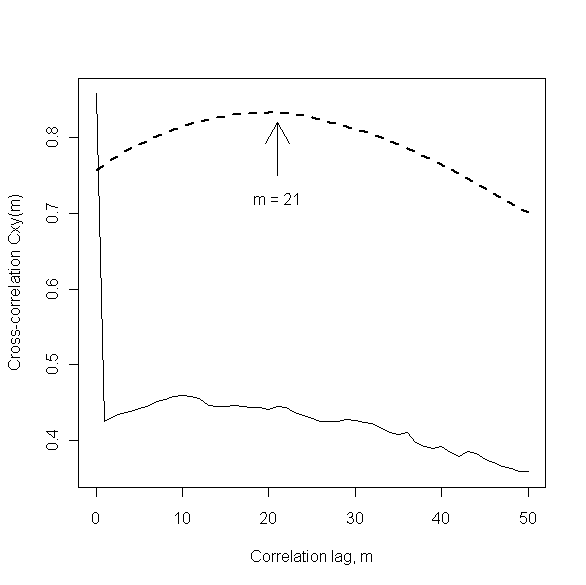
This example is discussed in more detail in Section 8.1.2 of my book Discrete-Time Dynamic Models, but the key observations here are the following.  First, the large spikes seen in both of the original data sequences were caused by the simultaneous, temporary loss of both measurements and the subsequent coding of these missing values as zero by the data collection system.  The practical question of interest was to determine how long, on average, the viscous, polymeric material being fed into and out of the product storage tank was spending there.  A standard method for addressing such questions is the use of cross-correlation analysis, where the expected result is a broad peak like the heavy dashed line in the plot shown below.  The location of this peak provides an estimate of the average time spent in the tank, which is approximately 21 hours in this case, as indicated in the plot.  This result was about what was expected, and it was obtained by applying standard cross-correlation analysis to the cleaned data sequences shown in the bottom two plots above.  The lighter solid curve in the plot below shows the results of applying exactly the same analysis, but to the original data sequences instead of the cleaned data sequences.  This dramatically different plot suggests that the material is spending very little time in the storage tank: accepted uncritically, this result would imply severe fouling of the tank, suggesting a need to shut the process down and clean out the tank, an expensive and labor-intensive proposition.  The main point of this example is that the difference in these two plots is entirely due to the extreme data anomalies present in the original time-series.  Additional examples of problems caused by time-series outliers are discussed in Section 4.3 of my book Mining Imperfect Data. 

           

One of the primary features of the analysis of time-series and other streaming data sequences is the need for local data characterizations.  This point is illustrated in the plot below, which shows the first 200 observations of the storage tank inlet data sequence discussed above.  All of these observations but one are represented as open circles in this plot, but the data point at k = 110 is shown as a solid circle, to emphasize how far it lies from its immediate neighbors in the data sequence.  It is important to note that this point is not anomalous with respect to the overall range of this data sequence – it is, for example, well within the normal range of variation seen for the points from about k = 150 to k = 200 – but it is clearly anomalous with respect to those points that immediately precede and follow it.  A general strategy for automatically detecting and removing such spikes from a data sequence like this one is to apply a moving window data cleaning filter which characterizes each data point with respect to a local neighborhood of prior and subsequent samples.  That is, for each data point k in the original data sequence, this type of filter forms a cleaned data estimate based on some number J of prior data values (i.e., points k-J through k-1 in the sequence) and, in the simplest implementations, the same number of subsequent data values (i.e., points k+1 through k+J in the sequence).

           

The specific data cleaning filter considered here is the Hampel filter, which applies the Hampel identifier discussed in Chapter 7 of Exploring Data in Engineering, the Sciences and Medicine to this moving data window.  If the k^th data point is declared to be an outlier, it is replaced by the median value computed from this data window; otherwise, the data point is not modified.  The results of applying the Hampel filter with a window width of J = 5 to the above data sequence are shown in the plot below.  The effect is to modify three of the original data points – those at k = 43, 110, and 120 – and the original values of these modified points are shown as solid circles at the appropriate locations in this plot.  It is clear that the most pronounced effect of the Hampel filter is to remove the local outlier indicated in the above figure and replace it with a value that is much more representative of the other data points in the immediate vicinity.

           

As I noted above, the Hampel filter implementation used here is that available in the R package pracma as procedure outlierMAD.  I will discuss this R package in more detail in my next post, but for those seeking a more detailed discussion of the Hampel filter in the meantime, one is freely available on-line in the form of an EDN article I wrote in 2002, Scrub data with scale-invariant nonlinear digital filters.  Also, comparisons with alternatives like the standard median filter (generally too aggressive, introducing unwanted distortion into the “cleaned” data sequence) and the center-weighted median filter (sometimes quite effective) are presented in Section 4.2 of the book Mining Imperfect Data  mentioned above.